Как реализовать базовые алгоритмы машинного обучения с нуля с Python
Дата публикации 2016-10-21
Важно установить базовую производительность по проблеме прогнозного моделирования.
Базовая линия обеспечивает точку сравнения для более продвинутых методов, которые вы оцените позже.
В этом руководстве вы узнаете, как реализовать базовые алгоритмы машинного обучения с нуля в Python.
После завершения этого урока вы узнаете:

Описание
Есть много алгоритмов машинного обучения на выбор. Сотни на самом деле.
Вы должны знать, хороши ли прогнозы для данного алгоритма или нет. Но как ты узнал?
Ответ заключается в использовании базового алгоритма прогнозирования. Алгоритм базового прогнозирования предоставляет набор прогнозов, которые вы можете оценить так же, как и любые прогнозы для вашей проблемы, такие как точность классификации или RMSE.
Оценки по этим алгоритмам обеспечивают требуемую точку сравнения при оценке всех других алгоритмов машинного обучения по вашей проблеме.
Установив это, вы можете прокомментировать, насколько лучше данный алгоритм по сравнению с наивным базовым алгоритмом, предоставив контекст о том, насколько хорош данный метод на самом деле.
Два наиболее часто используемых базовых алгоритма:
Когда вы начинаете с новой проблемы, которая является более сложной, чем обычная проблема классификации или регрессии, хорошей идеей будет сначала разработать алгоритм случайного прогнозирования, который является специфическим для вашей проблемы прогнозирования. Позже вы можете улучшить это и разработать алгоритм с нулевым правилом.
Давайте реализуем эти алгоритмы и посмотрим, как они работают.
Руководство
Этот урок разделен на 2 части:
Эти шаги обеспечат основы, необходимые для реализации и расчета базовой производительности для ваших алгоритмов машинного обучения.
1. Алгоритм случайного прогнозирования
Алгоритм случайного предсказания предсказывает случайный результат, как это наблюдается в данных обучения.
Это, пожалуй, самый простой алгоритм для реализации.
Это требует, чтобы вы сохранили все отдельные значения результатов в данных обучения, которые могут быть большими при проблемах регрессии с большим количеством различных значений.
Поскольку для принятия решений используются случайные числа, рекомендуется зафиксировать начальное число случайных чисел перед использованием алгоритма. Это сделано для того, чтобы мы получали одинаковый набор случайных чисел и, в свою очередь, принимали одинаковые решения при каждом запуске алгоритма.
Ниже приведена реализация алгоритма случайного прогнозирования в функции с именемrandom_algorithm (),
Функция принимает как обучающий набор данных, который включает выходные значения, так и тестовый набор данных, для которого выходные значения должны быть предсказаны.
Функция будет работать для задач классификации и регрессии. Предполагается, что выходное значение в обучающих данных является последним столбцом для каждой строки.
Во-первых, набор уникальных выходных значений собирается из обучающих данных. Затем случайно выбранное выходное значение из набора выбирается для каждой строки в тестовом наборе.
Мы можем проверить эту функцию с небольшим набором данных, который содержит только выходной столбец для простоты.
Выходные значения в обучающем наборе данных: «0» или «1», что означает, что набор прогнозов, из которых будет выбирать алгоритм, равен <0, 1>. Набор тестов также содержит один столбец без данных, поскольку прогнозы не известны.
Выполнение примера вычисляет случайные прогнозы для тестового набора данных и печатает эти прогнозы.
Алгоритм случайного прогнозирования прост в реализации и быстр в запуске, но мы могли бы добиться большего успеха в качестве базовой линии.
2. Алгоритм нулевого правила
Алгоритм нулевого правила является лучшей базовой линией, чем случайный алгоритм.
Он использует больше информации о данной проблеме, чтобы создать одно правило для прогнозирования. Это правило отличается в зависимости от типа проблемы.
Давайте начнем с проблем классификации, предсказания метки класса.
классификация
Для задач классификации одно правило состоит в том, чтобы предсказать значение класса, которое является наиболее распространенным в наборе обучающих данных. Это означает, что если в учебном наборе данных имеется 90 экземпляров класса «0» и 10 экземпляров класса «1», он будет прогнозировать «0» и достигать базовой точности 90/100 или 90%.
Это намного лучше, чем алгоритм случайного предсказания, который в среднем достиг бы точности всего 82%. Подробнее о том, как рассчитывается эта оценка для случайного поиска, см. Ниже:
Ниже приведена функция с именемzero_rule_algorithm_classification ()который реализует это для случая классификации
Функция используетМаксимум()Функция с атрибутом ключа, который немного умный.
Учитывая список значений класса, наблюдаемых в данных обучения,Максимум()Функция принимает набор уникальных значений класса и вызывает счетчик в списке значений класса для каждого значения класса в наборе.
В результате он возвращает значение класса с наибольшим количеством наблюдаемых значений в списке значений класса, наблюдаемых в наборе обучающих данных.
Если все значения классов имеют одинаковое количество, то мы выберем первое значение класса, наблюдаемое в наборе данных.
После того, как мы выбрали значение класса, оно используется для прогнозирования каждой строки в наборе тестовых данных.
Ниже приведен рабочий пример с надуманным набором данных, который содержит 4 примера класса «0» и 2 примера класса «1». Мы ожидаем, что алгоритм выберет значение класса «0» в качестве прогноза для каждой строки в тестовом наборе данных.
Выполнение этого примера делает прогнозы и выводит их на экран. Как и ожидалось, значение класса «0» было выбрано и предсказано.
Теперь давайте рассмотрим алгоритм нулевого правила для задач регрессии.
регрессия
Проблемы регрессии требуют предсказания реальной стоимости.
Хорошим прогнозом по умолчанию для реальных значений является прогнозирование центральной тенденции. Это может быть среднее или медиана.
Хорошим значением по умолчанию является использование среднего значения (также называемого средним) выходного значения, наблюдаемого в данных обучения.
Вероятно, это будет иметь меньшую погрешность, чем случайный прогноз, который вернет любое наблюдаемое выходное значение.
Ниже приведена функция для этогоzero_rule_algorithm_regression (), Он работает путем расчета среднего значения для наблюдаемых выходных значений.
После расчета среднее значение прогнозируется для каждой строки в данных обучения.
Эта функция может быть проверена на простом примере.
Мы можем создать небольшой набор данных, в котором среднее значение, как известно, равно 15.
Ниже приведен полный пример. Мы ожидаем, что среднее значение 15 будет предсказано для каждой из 4 строк в тестовом наборе данных.
При выполнении примера вычисляются прогнозируемые выходные значения, которые будут напечатаны. Как и ожидалось, среднее значение 15 прогнозируется для каждой строки в тестовом наборе данных.
расширения
Ниже приведены несколько расширений базовых алгоритмов, которые вы, возможно, захотите исследовать, как дополнение к этому учебнику.
Обзор
В этом руководстве вы узнали о важности расчета базового показателя производительности для вашей проблемы машинного обучения.
У вас есть вопросы?
Задайте свои вопросы в комментариях, и я сделаю все возможное, чтобы ответить.
Статический анализ: baseline файлы vs diff
В статических анализаторах рано или поздно приходится решать задачу упрощения интеграции в существующие проекты, где поправить все предупреждения на legacy коде невозможно.
Эта статья — не помощник по внедрению. Мы будем говорить о технических деталях: как такие механизмы подавления предупреждений реализуются, какие у разных способов плюсы и минусы.

baseline или так называемый suppress profile
Этот метод имеет несколько названий: baseline файл в Psalm и Android Lint, suppress база (или профиль) в PVS-Studio, code smell baseline в detekt.
Данный файл генерируется линтером при запуске на проекте:
Внутри себя он содержит все предупреждения, которые были выданы на этапе создания.
Прямолинейный подход, где предупреждения сохраняются целиком вместе с номером строки будет работать недостаточно хорошо: стоит добавить новый код в начало файла, как все строки вдруг перестанут совпадать и вы получите все предупреждения, которые планировалось игнорировать.
Обычно, мы хотим достичь следующего:
То, что мы можем конфигурировать в этом подходе — это какие поля предупреждения формируют хеш (или «сигнатуру») срабатывания. Чтобы уйти от проблем смещения строк кода, лучше не добавлять номер строки в эти поля.
Вот примерный список того, что вообще может являться полем сигнатуры:
Чем больше признаков, тем ниже риск коллизии, но при этом выше риск неожиданного срабатывания из-за инвалидации сигнатуры. Если любой из используемых признаков в коде изменяется, предупреждение перестанет игнорироваться.
PVS-Studio, в добавок к основной строке исходного кода добавляет предыдущую и следующую. Это помогает лучше идентифицировать строку кода, но при этом предупреждения на какую-то строку кода могут выдаваться из-за того, что вы редактировали соседнюю строку.
Ещё один менее очевидный признак — имя функции или метода, в которой выдавалось предупреждение. Это позволяет снизить количество коллизий, но провоцирует шквал предупреждений на всю функцию, если вы её переименуете.
Эмпирически проверено, что с этим признаком можно ослабить поле имени файла и хранить только базовое имя вместо полного пути. Это позволяет перемещать файлы между директориями без инвалидации сигнатуры. В языках, типа C#, PHP или Java, где название файла чаще всего отражает название класса, такие переносы имеют смысл.
Хорошо подобранный набор признаков увеличивает эффективность baseline подхода.
Коллизии в методе baseline
Допустим, диагностика W104 находит вызовы die в коде.
В проверяемом проекте есть файл foo.php :
Наш анализатор при создании baseline добавляет вызов die(‘test’) в свою базу исключений:
Теперь добавим немного нового кода:
По всем используемым признакам новый вызов die(‘test’) будет распознаваться как игнорируемый код. Совпадение сигнатур для потенциально разных кусков кода мы и называем коллизией.
Одним из решений является добавление дополнительного признака, который позволит различать эти вызовы. К примеру, это может быть поле «имя содержащей функции».
Что делать, если вызов die(‘test’) был добавлен в ту же функцию? Этот вызов может иметь одинаковые соседние строки в обоих случаях, поэтому добавление предыдущей и следующей строки в сигнатуре не поможет.
Здесь нам на помощь приходит счётчик сигнатур с коллизиями. Таким образом мы можем определить, что внутри функции ожидалось одно срабатывание, а получили два или более — все, кроме первого, нужно сообщать.
При этом мы теряем некоторую точность: нельзя определить, какая из строк новая, а какая — старая. Мы будем ругаться на ту, что будет идти после проигнорированных.
Метод, основанный на diff возможностях VCS
Исходной задачей было выдавать предупреждение только на «новый код». Системы контроля версий как раз могут нам в этом помочь.
Утилита revgrep принимает на stdin поток предупреждений, анализирует git diff и выдаёт на выход только те предупреждения, которые исходят от новых строк.
golangci-lint использует форк revgrep как библиотеку, так что в основе его вычисления diff’а лежат те же алгоритмы.
Если выбран этот путь, придётся искать ответ на следующие вопросы:
Нам нужно не только получить правильный набор затронутых строк, но и расширить его так, чтобы найти побочные эффекты изменений во всём проекте.
Окно коммитов тоже можно определить по-разному. Скорее всего, вы не захотите проверять только последний коммит, потому что тогда будет возможно пушить сразу два коммита: один с предупреждениями, а второй — для обхода CI. Даже если это не будет происходить умышленно, в системе появляется возможность пропустить критический дефект. Также стоит учесть, что предыдущий коммит может быть взят из основной ветки, в этом случае проверять его тоже не следует.
diff режим в NoVerify
NoVerify имеет два режима работы: diff и full diff.
Обычный diff может найти предупреждения по файлам, которые были затронуты изменениями в рамках рассматриваемого диапазона коммитов. Это работает быстро, но хорошего анализа зависимостей изменений не происходит, поэтому новые предупреждения из незатронутых файлов мы найти не можем.
Full diff запускает анализатор дважды: один раз на старом коде, затем на новом коде, а потом фильтрует результаты. Это можно сравнить с генерацией baseline файла на лету с помощью того, что мы можем получить предыдущую версию кода через git. Ожидаемо, этот режим увеличивает время выполнения почти вдвое.
Изначальная схема работы предполагалась такая: на pre-push хуках запускается более быстрый анализ, в режиме обычного diff’а, чтобы люди получали обратную связь как можно быстрее. На CI агентах — полный diff. В результате время от времени люди спрашивают, почему на агентах проблемы были найдены, а локально — всё чисто. Удобнее иметь одинаковые процессы проверки, чтобы при прохождении pre-push хука была гарантия прохождения на CI фазы линтера.
full diff за один проход
Мы можем делать приближенный к full diff аналог, который не требует двойного анализа кода.
Допустим, в diff попала такая строка:
Если мы попробуем классифицировать эту строку, то определим её как «Foo class deletion».
Каждая диагностика, которая может как-то зависеть от наличия класса, должна выдавать предупреждение, если имеется факт удаления этого класса.
Аналогично с удалениями переменных (глобальных или локальных) и функций, мы генерируем набор фактов о всех изменениях, которые можем классифицировать.
Переименования не требуют дополнительной обработки. Мы считаем, что символ со старым именем был удалён, а с новым — добавлен:
Основной сложностью будет правильно классифицировать строки изменений и выявить все их зависимости, не замедлив алгоритм до уровня full diff с двойным обходом кодовой базы.
Выводы
baseline: простой подход, который используется во многих анализаторах. Очевидным недостатком данного подхода является то, что этот baseline файл нужно будет где-то разместить и, время от времени, обновлять его. Точность подхода зависит от удачного подбора признаков, определяющих сигнатуру предупреждения.
diff: прост в базовой реализации, сложен при попытках достичь максимального результата. В теории, этот подход позволяет получить максимальную точность. Если ваши клиенты не используют систему контроля версий, то интегрировать ваш анализатор они не смогут.
| baseline | diff |
|---|---|
| + легко сделать эффективным | + не требует хранить файл исключений |
| + простота реализации и конфигурации | + проще отличать новый код от старого |
| — нужно решать коллизии | — сложно правильно приготовить |
Могут существовать гибридные подходы: сначала берёшь baseline файл, а потом разрешаешь коллизии и вычисляешь смещения строк кода через git.
Лично для меня, diff режим выглядит более изящным подходом, но однопроходная реализация полного анализа может оказаться слишком затруднительной и хрупкой.
Machine Learning Blog | ML@CMU | Carnegie Mellon University
Statistics:
Categories:
3 – Baselines
Authors
Affiliations
Published

Figure 1. The diagram is a metaphor which demonstrates how “good” results can be misleading if we compare against a weak baseline. A seemingly optimistic progress may be illusory because of a weak baseline, just like a chain may be vulnerable when a single link is weak. Hence, we need to be extra cautious when we show improvements over a baseline as those improvements may not be warranted.
Introduction
Assume you work for an apparel retailer as a data scientist and your task is to send out 100,000 advertising mail pieces to past customers about a new line of fall apparel. You have access to a database of information about past customers, including what they have purchased and their demographic information (Ramakrishnan 2018). What model should you build first?
In this article, we will discuss what a baseline is and where it fits in our data analysis projects. We will see that there are two different types of baselines, one which refers to a simple model, and another which refers to the best model from previous works. A baseline guides our selection of more complex models and provides insights into the task at hand. Nonetheless, such a useful tool is not easy to handle. A literature review (Lin 2019; Mignan 2019; Rendle et al. 2019; Yang et al. 2019) shows that many researchers tend to compare their novel models against weak baselines which poses a problem in the current research sphere as it leads to optimistic, but false results. A discussion on such contemporary issues and open-ended questions is also provided at the end, followed by suggestions aimed at the community.
Baselines in Problem Solving – Overview
People use data analysis techniques to solve practical problems that may or may not require deep understanding of machine learning algorithms. Common-sense models that act as baselines in many cases perform surprisingly well compared to complicated machine learning models.
What is a baseline?
A baseline is a simple model that provides reasonable results on a task and does not require much expertise and time to build. Common baseline models include linear regression when predicting continuous values, logistic regression when classifying structured data, pretrained convolutional neural networks for vision related tasks, and recurrent neural networks and gradient boosted trees for sequence modeling (Ameisen 2018).
Because it is simple, a baseline is not perfect. For example, the bag of words model for language modeling does not take into account the order of the words occurring in each sentence, hence, it is missing out on a lot of structural information. Also, many baselines largely depend on heuristics embedded in the model or on strong modelling assumptions (i.e. linear models). Finally, from a researcher’s perspective, a baseline does not provide cutting-edge research experience which makes it harder to publish.
If baselines are not perfect, then what makes them useful? Let’s circle back to the apparel example. Common sense tells us to mail the top 100k loyal customers to maximize our expected return. Loyalty can be measured in terms of three features. If customers shop a lot, spend a lot, and have recently shopped with your store, then they are likely to be loyal (Ramakrishnan 2018). One way to combine these three pieces of information is binning, where we categorize each customer for each category and then simply rank them based on some scale. The top 100k customers are the ones you should mail. In fact, this model is a practical heuristic, called the Recency-Frequency-Monetary Heuristic, which is commonly used in database marketing and direct marketing. It is easy to create, easy to explain, easy to use, and effective.
Why start with a baseline?
A baseline takes only 10% of the time to develop, but will get us 90% of the way to achieve reasonably good results. Baselines help us put a more complex model into context in terms of accuracy. Ameisen (2018) names four levels of performance we can categorize a model into. Using these levels of performance we can determine what level we want our model to achieve based on our domain knowledge, our computational and human resources, and our business goals. Each level of performance will guide our selection of a baseline.
Another advantage of a baseline is that it’s easy to deploy, it is faster to train as few parameters can quickly fit to your data, and it is often simple enough to allow easy problem detection. Whenever an error pops up, it is likely due to a bug, some defect of the dataset, or due to wrong assumptions. A baseline is quick to put into production as it does not require much infrastructure engineering, and it is also quick for inference because it has low latency.
What to do after building a baseline?
Having constructed a baseline, the next step is to see what the baseline fails to capture. This will guide our choice of a more complex model. That being said, we should also not neglect the fact that improving upon baselines can make already successful cases fail, as improvements are not strictly additive. This is especially true in the case of deep learning models where the lack of interpretability makes it harder to infer failure cases.
Furthermore, baselines help us understand our data better. For example, for a classification task we can get an idea of what classes are hard to separate from each other by looking at the confusion matrix. If we have a lasso regression problem, we can look at the non-zero coefficients to guide feature selection. Furthermore, if the model neglects some features that our domain knowledge tells us are important, then that sends a warning signal as our data may not be a good representation of the population or it could just be that the model is not suitable.
Baselines in Research – Weak Baselines
Now that we have an idea of what baselines are, let us shift our attention to how they have been used in academia. Great expectations surround AI and Machine Learning about their role in changing the world. The past few years have witnessed an increase in research output and empirical advancement in all Machine Learning related areas. However, this increase has not necessarily been matched with a rigorous analysis of the underlying methods. This has led to a gap between the level of empirical advancement and the level of empirical rigor which is partly due to the research culture that our community has developed; a culture that rewards “wins” which usually means beating a previous method on some task (Lin 2019). While there seems to be nothing wrong with this culture, issues emerge when it is the authors themselves who determine what previous method to compare against. For many, a “win” means beating a baseline, even if that baseline is weak. The following examples support this claim.
Netflix vs Movielens
Before we discuss “wins” we need to have a clear understanding of what it means for a baseline to be good. Rendle et al. (2019) show that measuring the performance of a baseline model for a particular task is not as straightforward as it might first seem. In their work, they refer to two extensively studied datasets, Movielens and Netflix, to indicate that running baselines properly is difficult.
The Movielens datasets are widely used in recommender systems research. Over the past five years, numerous new recommendation algorithms have been published, reporting large improvements over baseline models such as Bayesian MF, RSVD, and BPMF, as reported in Figure 2. Rendle et al. (2019) show that these baselines can beat the current state-of-the-art models on this benchmark just by tuning the baselines and combining them with simple, well-known methods. Furthermore, Bayesian MF, which was previously reported to perform poorly, after proper tuning is able to outperform any results reported on this benchmark so far.
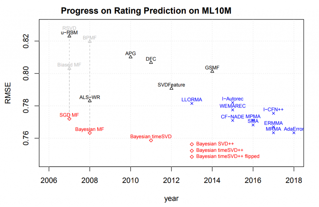
Figure 2. Rerunning baselines for Bayesian MF and other popular methods, where results marked in blue crosses were reported by the corresponding researchers and those marked as black triangles were run as baselines. Lower is better. After additional tuning, these baselines (marked in red) can achieve much better results than previously reported methods. Table borrowed from Rendle et al. (2019).
The Netflix Challenge also demonstrates that running methods properly is hard. The Netflix Prize was awarded to the team who improved Netflix’s own recommender system by 10%. From the beginning of this competition, matrix factorization algorithms were widely used as baselines. Authors show some key results for vanilla matrix factorization models reported by top competitors and winners, and there is a steady progress on the different methods based on the same baseline. This indicates that achieving good results even for a presumably simple method like matrix factorization is a non-trivial task and takes time and effort.
These findings on the differences between Movielens and Netflix datasets question the current results of the baseline models as well as any newly proposed methods. Even though these results follow good practices (conducting a reasonable hyperparameter search, reporting statistical significance and allowing reproducibility), they are still sub-optimal (Rendle et al. 2019).
Weak Baselines in Information Retrieval
A similar example is presented by Lin, a professor at the University of Waterloo, who decided to test the effectiveness of some well-known, albeit old, ranking algorithms against two recently published papers that appear at top Information Retrieval conferences (2019). The old ranking algorithms have served as baselines for years, however, there has not been much interest in tuning them and discovering their full potential. What Lin discovers is that by exploring their hyperparameters via a simple grid search, one can find much better-performing baselines which nullify the improvements of the other novel methods.
Lin considers variants of BM25, Query Likelihood with Dirichlet Smoothing (QL) and RM3 as possible baselines and compares them against the reported performances in Paper 1 and Paper 2. Figure 3 lists the results.
Both Paper 1 and Paper 2 suffer from similar problems – weak baselines. Lin reports that the authors of Paper 1 do a good job tuning the baseline they use (QL). What they fail to do is consider other baselines which may potentially result in better performances. In this particular case, BM25+RM3 matches the performance of Model 1, rendering its claimed improvements invalid. Paper 2, on the other hand, uses an untuned version of BM25 and the tuned baseline surpasses Model 2 by a fair margin, which raises the question whether they are really making progress (Lin 2019).
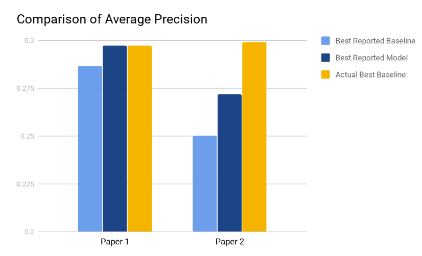
Figure 3. The chart compares the reported average precision (AP) of the baselines and the contributions of both Paper 1 and Paper 2 versus the AP of the tuned baselines. Results from Lin (2019).
Yang et al. take this issue to the next level and ask if such comparisons are common practice among other researchers (2019). They survey a multitude of papers in Information Retrieval to shed some light into this question. The results are deeply troubling. Figure 4 plots the average precision for every baseline used in the surveyed papers alongside that paper’s contributed performance. It is worth noting that, not only the baselines, but also 60% of the proposed models perform worse than an untuned RM3 (dashed black line). Furthermore, only six papers “win” over the best performing model of 2004 (solid black line), and out of those, five papers are more than a decade old. As Lin puts it, the more alarming fact is that this trend has gone largely unnoticed by the community (2019).
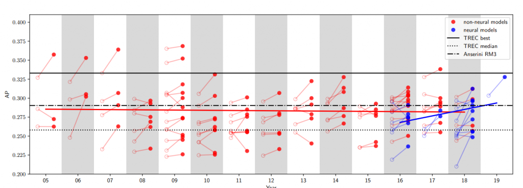
Figure 4. Average Precision of the baselines used in the papers surveyed by Yang et al. versus the year they were published. Empty circles represent the baseline and the linked red circles represents the contributed performance. Table borrowed from Yang et al (2019).
Nonetheless, this does not mean that the past decade has not witnessed any progress. It is sometimes acceptable to achieve similar or worse performances if it means trading that bit of accuracy for more robustness or interpretability. While the survey done above considers only the rates of average precision reported, it does not survey the novelty scores and contributions that these papers may have. Therefore, these results are somewhat overly pessimistic and should be taken with a grain of salt.
Construction and Improvement of Baselines
A recent paper, published in Nature by DeVries et al (2018), proposed a deep neural network (DNN) with 13k parameters to forecast aftershock locations in the aftermath of large seismic events. Interestingly, this DNN is outperformed by a much simpler baseline model. Mignan and Broccardo replicate these results by using a two-parameter logistic regression (2019). This demonstrates that the proposed deep learning strategy does not provide any new insights.
How can we avoid this mistake?
Improving Baselines Strategically
These ideas were originally presented in Merity (2017).
Discussion
Now that we’ve discussed how to get the baseline right and strong, one question we should ask ourselves is how much complexity should we add to a baseline?
Baseline Complexity Revisited
Suppose we are doing sequence modeling in a research setting. Our baseline methods include a traditional recurrent neural network (RNN) and our novel model is based on the state-of-the-art transformer model. When we compare these models for a generation task, we consider the option of adding beam search to our modified transformer model. Should we also add beam search to the baseline RNN model? If we do not, is the comparison fair? On the other hand, if we do, is RNN still a baseline?
This question leads to two different notions of baselines. One is the baseline we use in problem solving, where we defined it to be a very simple method that is known to perform reasonably well at some task. The second kind is the baseline models that we use in research, such as the current state-of-the-art models. This serves the purpose of showing that our novel models are performing better. It’s important to be able to distinguish between these two use cases of baselines.
We have seen through the Movielens and IR examples how using an untuned baseline leads to issues in model comparison. In case we decide to use the second notion of a baseline, that of the current state-of-the-art, a follow up question could be “should we tune the state-of-the-art?” The answer depends. If we enhance our proposed models with general techniques such as regularization techniques like dropout or weight decay, then we should also implement them for the baseline for a fair comparison. Most importantly, although the ML community tends to criticize incremental improvements of already existing models, empirical results are still needed to explore different combinations of techniques to analyze and better understand their interactions.
In a Reddit thread (radarsat1 2019) that discusses the 2 parameter logistic regression versus a 13k deep learning model on aftershock prediction, we found a comment that made a good point. In essence, the commenter drew a comparison between statistics and deep learning. More specifically, he argues that both statisticians and deep learning engineers make claims based on experimental results, but statisticians have a rigorous process to show something is statistically significant with a certain confidence interval. The same question can be asked regarding baselines, namely how can we rigorously show that our complex models are doing better than the baselines? A look at the accuracy bar does not suffice to answer this question. When designing a new model, we should be constantly aware that we are not building a complex model for the sake of its complexity but for its expressiveness. Our inability to address this issue on both the intuitive and theoretical level is an intellectual debt that we will eventually need to pay off.
A Community Approach
The examples we have listed so far do not only suggest a problem with a specific group of self-centered researchers, but a problem with the entire community and the way the community assesses productivity. If papers that report comparisons against weak baselines keep getting accepted into top conferences, then perhaps the community is as guilty as the authors. Therefore, fundamental changes are needed in order to build a more serious and flourishing community of researchers. We suggest the following ideas borrowed from Lin (2019).
Nonetheless, no solution is perfect and there are issues that arise with each recommendation. For example, it is not clear how one determines what a strong baseline is if the research area is exotic and the number of researchers is limited. A leaderboard would fail in this case, and publishing committees would face a much harder task at validating the baselines used. Similarly, datasets such as those in medicine are usually private, making it infeasible to construct a good public baseline. In that case, we have no choice but to trust the owners of the dataset in their rigor. Finally, using a centric leaderboard may lead to issues of overfitting to the dataset, as all researchers will be comparing against the same baseline and that is also undesirable.
Conclusion
We have seen that a baseline is an important component of a data analysis project. A baseline helps us understand the task better, helps us discover inconsistencies with the data, and gets us up and running in no time. However, the use of a weak baseline may lead to the false belief that some methods are performing well when they are not, which hinders development and progress. Hence, we need to be cautious about the baseline we use and the amount of effort we pay to tuning. Finally, we should be aware that such weak comparisons are not solely the researchers’ fault, but they suggest a defect in the way we do research as a community, which calls for changes from above. This will ultimately lead to a healthier research environment which appreciates good knowledge.
Sources
DeVries, Phoebe MR, et al. “Deep learning of aftershock patterns following large earthquakes.” Nature 560.7720, (2018): 632.
Mignan, A., and M. Broccardo. “One neuron versus deep learning in aftershock prediction.” Nature 574.7776 (2019).
Rendle, Steffen, Li Zhang, and Yehuda Koren. “On the Difficulty of Evaluating Baselines: A Study on Recommender Systems.” arXiv preprint arXiv:1905.01395 (2019).
Yang, Wei, et al. “Critically Examining the “Neural Hype”: Weak Baselines and the Additivity of Effectiveness Gains from Neural Ranking Models.” (2019), pp. 2–5.